Conducting Simple Linear Regressions in R

Israel Arevalo 2023-01-22

• Data Preparation
• Conducting a Simple Linear Regression
• Model Summary
• Visualizing the Results

Simple linear regression is a statistical method used to model the relationship between a single independent variable and a single dependent variable. In R, the lm() function can be used to fit a simple linear regression model. In this tutorial, we will use simulated educational data to demonstrate how to conduct a simple linear regression in R.

As in previous guides, several assumptions about the user will be made.

1. You have installed R and an IDE such as RStudio on your computer
2. You have a dataset to work with (we will generate a dataset in this tutorial but you will need a dataset to run your own analysis outside of the tutorial, of course)

For additional information, please follow the links below as necessary.

• Installing RStudio
• Exporting SPSS dataset to .CSV
• Exporting STATA dataset to .csv
• Exporting Excel file to .csv

Data Preparation

First, we will need to load in the necessary packages and create the simulated data set. For this tutorial, we will create a data set that contains information on students’ math scores and the number of hours they study per week.

# Loading Packages
library(ggplot2)

set.seed(12314)  # for reproducibility

# create the data set (this data is purposefully manipulated to yield significant results for the purpose of the tutorial)
data <- data.frame(student_id = 1:30,
                   math_score = rnorm(30, mean = 70, sd = 10),
                   study_hours = rnorm(30, mean = 10, sd = 2))

Next, we will take a look at the structure of the data set using the str() function.

str(data)

## 'data.frame':    30 obs. of  3 variables:
##  $ student_id : int  1 2 3 4 5 6 7 8 9 10 ...
##  $ math_score : num  75 75.3 73 71 81.6 ...
##  $ study_hours: num  9.28 13.21 10.59 7.94 10.79 ...
Copy

Conducting a Simple Linear Regression

Now that we have the data loaded, we can fit a simple linear regression model using the lm() function. The function takes the form lm(y ~ x, data), where y is the dependent variable and x is the independent variable.

model <- lm(math_score ~ study_hours, data = data)

The output of this function is a linear model object that contains the coefficients of the model, the residuals, and other information.

Model Summary

We can use the summary() function to get a summary of the model and see the coefficients of the model.

summary(model)

## 
## Call:
## lm(formula = math_score ~ study_hours, data = data)
## 
## Residuals:
##      Min       1Q   Median       3Q      Max 
## -18.5178  -5.3500   0.9746   5.3003  13.2727 
## 
## Coefficients:
##             Estimate Std. Error t value Pr(>|t|)    
## (Intercept)   86.013      6.646  12.943 2.45e-13 ***
## study_hours   -1.516      0.656  -2.311   0.0284 *  
## ---
## Signif. codes:  0 '***' 0.001 '**' 0.01 '*' 0.05 '.' 0.1 ' ' 1
## 
## Residual standard error: 8.637 on 28 degrees of freedom
## Multiple R-squared:  0.1601, Adjusted R-squared:  0.1302 
## F-statistic: 5.339 on 1 and 28 DF,  p-value: 0.02843
Copy

This output is showing the results of a simple linear regression analysis, which is a statistical method used to model the relationship between a single independent variable study_hours and a single dependent variable math_score.

The first part of the output shows the residuals. Residuals are the differences between the observed values and the predicted values of the dependent variable. The Min, 1Q, Median, 3Q and Max values give an idea of the range and distribution of the residuals.

The second part of the output shows the coefficients of the model, including the intercept (the value of the dependent variable when the independent variable is 0) and the slope (the change in the dependent variable for a one-unit change in the independent variable). The estimate column shows the value of the coefficient, the Std. Error column shows the standard error of the estimate, the t value column shows the t-value, and the Pr(>|t|) column shows the p-value.

The p-value for the intercept and the slope is very small (2.45e-13 and 0.02843 respectively) which is less than 0.05. This means that the intercept and the slope are statistically significant. This means that, the relationship between math_score and study_hours is strong enough to say that there is a real relationship between them with a high degree of confidence.

The next value is the R-squared value which represents the proportion of the variance in the dependent variable that is predictable from the independent variable. In this case, the R-squared value is 0.1601, which is quite high, which means that the relationship between the two variables is strong.

Overall, the results show that the slope study_hours is statistically significant, this means that the number of hours studied per week is strongly related to the math scores. Therefore, the relationship between the two variables is strong and it is possible to make predictions about math scores based on the number of hours studied per week.

Visualizing the Results

Finally, we can create a scatter plot of the data with the line of best fit to visualize the relationship between the two variables.

ggplot(data, aes(x = study_hours, y = math_score)) +
  geom_point() +
  geom_smooth(method = "lm", color = "red") +
  ggtitle("Scatter plot of Math Scores vs Study Hours")

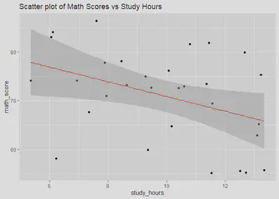
This plot shows the relationship between the math_score and study_hours variables, and can help to further illustrate the strength and direction of the relationship modeled by the linear regression. The line of best fit (in red) shows the direction of the relationship and the slope of the line represents the strength of the relationship.

In summary, this tutorial demonstrated how to conduct a simple linear regression using simulated educational data in R. The steps outlined in this tutorial can be applied to any data set and any set of variables. Simple linear regression is a useful tool for modeling the relationship between a single independent variable and a single dependent variable, and it can provide insights into the extent to which the independent variable is related to the dependent variable. Additionally, visualizing the results using the ggplot2 package can help to further understand the relationship between the variables.

Please keep in mind that this is a basic linear regression, and in practice, the data might be affected by other variables that can change the relationship between the dependent and independent variables. So, it’s important to consider other factors that may be impacting the relationship between the variables and use appropriate statistical methods accordingly. In practice, it is important to be mindful of extant literature to help guide your study from conceptualization to dissemination.